Well Diffracting Samples

Well diffracting samples are often trivial to peakfind and then index. These well behaved crystals also run fast with most modern peakfinding algorithms. Therefore, the essential question is if this method can match those from more established libraries.

Setting Up (FEL)

As always, we need to provide our expected cell, geometry, and a list file of files to index. We can additionally gather information about the noise model we are creating. probixi will try to read the pixel mask stored in .cxi files and then add other detected misbehaving pixels (if any). For this experiment, let’s go with bacterioRhodopsin.

probixi \
  -i lysozyme.lst \
  -g swissfel.geom \
  -p lysozyme.cell \
  -o lysozyme.stream \
  --device cuda \
  --gif noise_model.gif \
  --enrich-gate \
  --flux-variance

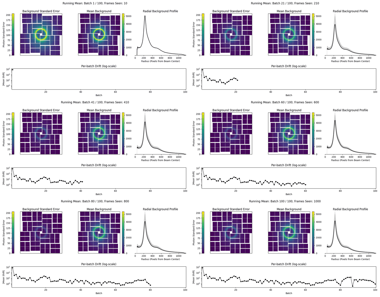
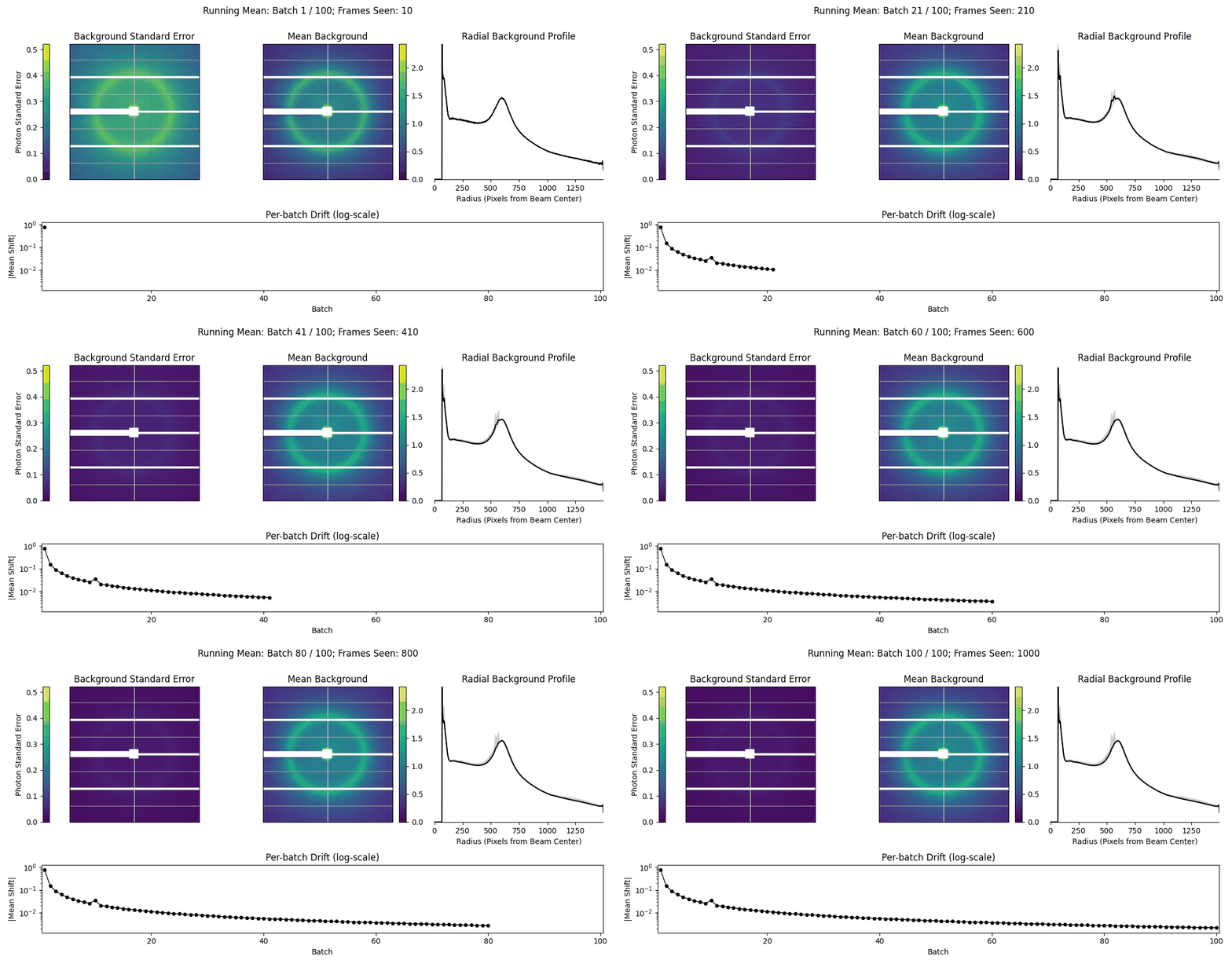
--gif noise_model.gif writes a diagnostic animation of the noise model as it warms over the seed frames — the running mean background, its radial profile, and the per-batch drift. It costs only a few seconds and is the quickest way to confirm the background and the learned dead-pixel mask have settled before you trust the detected peaks. Writing -o lysozyme.stream (rather than a .db) gives a CrystFEL-style stream you can feed straight into partialator/process_hkl next to an indexamajig run, so the two pipelines can be compared one-to-one on the same data.

NOTE: the .stream format may be deprecated in the future and exists now to compare end-of-pipeline results.

The enrichment gate

--enrich-gate is the one flag worth reaching for on strong data. Bright, well-diffracting shots produce many peaks, and with that many constraints it is occasionally possible to seed and refine an orientation that fits the peaks yet is not the true lattice – an overprediction that would quietly pollute the merge. The gate is a per-frame significance test that catches exactly this.

After a frame is indexed, probixi predicts the full lattice and asks a simple question of the image itself: of the predicted reflection positions, how many actually land on above-threshold signal? That count (n_bright) is compared to the rate at which any valid pixel clears the same threshold, giving

• an enrichment ratio, the bright-rate of predicted spots over the background bright-rate (≈ 1 for a chance/noise indexing, >> 1 for a genuine lattice), and

• a Poisson p-value (enrich_p) — the probability of seeing at least n_bright bright predicted spots by chance under that background.

--enrich-gate keeps only frames whose p-value falls below --enrich-alpha (default 1e-3); everything else is dropped as not backed by signal beyond chance. Because you are setting a false-discovery level rather than an enrichment cutoff, there is no magic number to retune per dataset — the test calibrates itself against each frame’s own background. That makes it a natural fit for high-fluence FEL data, where it removes misindexed strong shots without touching the good ones. Every predicted frame still carries its enrichment, n_bright, and enrich_p values in the output (see the frames table), so you can inspect or re-threshold the cut afterwards even without the gate enabled.

The photon-transfer curve

--flux-variance is the second flag worth enabling on FEL data, and for the same underlying reason: shot-to-shot fluence is not constant. At an XFEL the jet intensity swings from pulse to pulse, so one frame’s background can be several times brighter than the next. By default probixi whitens peaks against a single frozen variance floor learned during calibration — a reasonable per-pixel noise level, but one that assumes every frame sits near the calibration fluence. On a bright shot that floor understates the true noise (Poisson variance grows with signal, so brighter pixels are genuinely noisier), and on a dim shot it overstates it.

--flux-variance replaces that flat floor with a fitted photon-transfer curve. During calibration probixi regresses per-pixel variance against signal level across the seed frames and fits the classic linear relation

\[\mathrm{var} = \sigma_\text{read}^2 + g \cdot \text{level},\]

where the intercept is the read-noise variance and the slope g is the conversion gain. At detection time each pixel is then whitened against the noise it should have at its current signal level rather than a one-size-fits-all floor, so a bright jet shot and a dim one are judged on the same statistical footing. --flux-var-floor (default 0.15) still applies underneath as a fractional lower bound, guarding against pathologically small fitted variances. The recovered gain is also handed to the indexer, so integration downstream sees the same photon-scale calibration.

It is opt-in because it only helps when flux actually varies: on steady synchrotron exposures the frozen floor is already a good description of the noise, and the extra fit buys little. On jet-intensity-variable XFEL/SFX data it is the difference between a threshold that tracks each frame and one calibrated for the average frame.

Setting Up (Synchrotron)

Again, we provide our cell, geometry, and a list of files to index. In similar fashion to above, we can provide --enrich-gate which hones down our results and protects against overprediction. This time, let’s use BacterioRhodopsin taken at the synchrotron.

probixi \
  -i lysozyme_ssx.lst \
  -g synchrotron.geom \
  -p lysozyme.cell \
  -o lysozyme.stream \
  --device cuda \
  --enrich-gate

The calls are identical. Serial synchrotron shots are usually lower fluence than at an FEL, so per-frame signal is weaker. The self-calibrating noise model and detection threshold do that adapting for you. The enrichment gate applies unchanged, still guarding against the occasional overprediction on the strongest shots.